
Introduction
In the large amplitude oscillatory shear (LAOS) experiment, the material is deformed in its nonlinear viscoelastic regime. The information of nonlinear viscoelasticity can be extracted from the higher harmonic tones of the Fourier transform of the response. To date, different parameters were proposed to characterized many aspects of the nonlinear viscoelasticity under LAOS; among them widely used are
- the related intensity of higher harmonics, In/1,
- the shape parameters of the Lissajous curve, GM, GL and Gk.
For their definition and more detailed information of the LAOS rheology, please refer to the review by Hyun et al.[1].
R. Ewoldt et al. have written the MITlaos code specifically for the analysis of Lissajous curves and the Chebyshev coefficients. The code calculates the Lissajous parameters (alternative moduli) from the Fourier transformed harmonics instead of finding the slope of the curve as the definition of the parameters. The code is not compiled. My motivation is to design another tool for LAOS data analysis that
- complements the functions of MITlaos,
- allows the user to collect a series of results, e.g. a strain sweep test series, and
- provides a standalone .exe application for students who do not have a MATLAB suite.
How to use
Download the package here and extract all files to the same folder.
The tool runs on Windows 10 64-bit system with the MATLAB Compiler Runtime (MCR) installed. Please check the readme.txt file for the correct version of the MCR.
After installing the MCR, run the SCUT_LAOS.exe file, and the user interface looks like the figure below.
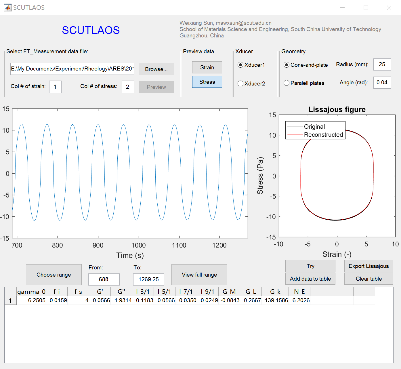
The interface of the LAOS tool (click to enlarge).
First, select the Xducer and enter the geometry information. This must be done before loading the data file; changing these fields after loading the data file takes no effect on the calculation and may lead to erroneous results1.
Second, click Browse… to select the data file to be analysis. The format of the data file should look like this:
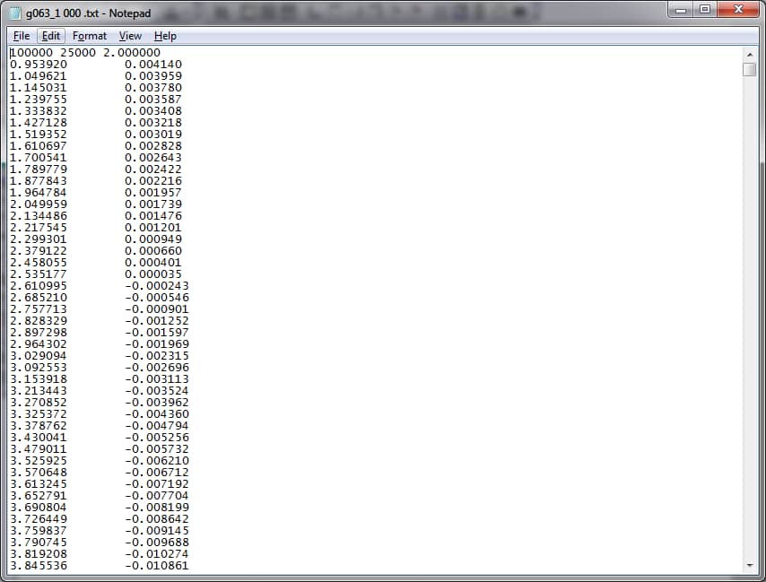
Input file format (click to enlarge).
The first row contain 3 parameters separated by spaces. The first parameter is the highest sampling frequency in Hz of the ADC. This parameter is not used by the software. The second parameter is the number of samples that are oversampled. The third parameter is the maximum frequency in Hz. The rest of the rows are the measured data separated by tab. The two columns should be the STRAIN and TORQUE voltage signals from the rear panel of the ARES rheometer.
This data format was generated by the LabView application (“FT_Measurement”) developed by the group of Prof. Manfred Wilhelm. For other users, just added a line of three parameters manually above the data. Select any values for the first two parameters so that the sampling frequency of the data = first parameter / second parameter (which is how the software will calculate the sampling frequency). The third parameter is not used by the tool so fill in any value, but don’t leave it blank.
Indicate the column number of the stress or strain at the specified text boxes (Col# for strain/stress). Click the “Preview” button and the signal will display in the plot below.
Third, click “Choose range” button, and the mouse pointer becomes a cross. In order to select a portion of signal, click once at the beginning, and click again on the end. The Lissajous curve of the selected portion will be plotted on the right. Click “View full range” button to return to the view of full signal. Click the “Strain” or “Stress” button above in the “Preview data” panel to alter between signals.
Forth, click “Try”, and the tool will attempt to reconstruct the selected range of signal. The result will be plotted on the right.
Briefly, the algorithm of the reconstruction starts from an exact coherent sampling of both signals. To achieve the exact coherent sampling, the actual frequency of the signals is first estimated by sine wave fitting using sinfapm coded by Miroslav Balda. After coherent sampling the signals, a Fourier transform is performed and the strain and stress signals are reconstructed by the harmonic tones. The first 25 harmonics or the maximum harmonic allowed by the sampling frequency according to the Nyquist-Shannon theorem are used for reconstruction. Any DC components in both signals are eliminated so the reconstructed signal may show some offset compared with the original ones. Sometimes the reconstructed Lissajous curve will look totally dislike the original signal (e.g. a much smaller circle than the original one). This may due to failure in the sine wave fitting step. If this happens, please check the noisiness of the strain signal. Select a smaller number of cycles will facilitate the sine wave fitting process if the strain signal is a little noisy. The software has difficulty in reconstruction if the strain signal is nearly pure noise.
If the reconstruction looks fine in the plot, you can click “Add data to table” button to temporally hold the results. The nonlinear viscoelastic parameters provided by the tool are shown in the header row of the table. fi is the frequency in Hz, and fs is the sampling frequency of the signal. The Lissajous parameters GM, GL and Gk (in Pa) are calculated by slope finding on the reconstructed signal. The slope finding is performed for all cycles and the results are averaged. These maximize the signal-to-noise ratio (SNR) of the results. The NE parameter was suggested by me [2]. Click Export Lissajous to export the re-construed data of the Lissajous curve. The exported file name will be the original data file name added by “_Lissajous.txt”. The file contains two columns of data. The first column is strain and the second is the stress.
Repeat step 1 to 4 for the next data file, and the new results will be appended to the table with the old data every time you click the “Add data to table” button. Finally select and copy all the data to another plotting software such as OriginPro or Excel. Click “Clear table” whenever needed. The LAOS analysis tool does not save or export any files.
Click the “x” button on the top-right to exit.
Example:
1. Perform a series of oscillatory time sweep with a fixed frequency (f = 1 Hz) and increasing strain amplitudes (γ0 = 4% ~ 160%) on ARES. Record the STRAIN and TORQUE votage signals of each time sweep to separated data files
2. Load the data files one by one in ascend order of strain amplitude and add data to table after construction in SCUT_LAOS. Also click Export Lissajous to get each reconstructed Lissajous curves of corresponding strain amplitudes
3. Copy the data to OriginPro and you have a column of strain amplitude for the x axis with a bunch of strain amplitude depending LAOS parameters. A strain sweep plot of any of these parameters can be plotted directly. Lissajous curves of any strain amplitude can be plotted from the exported files, too.
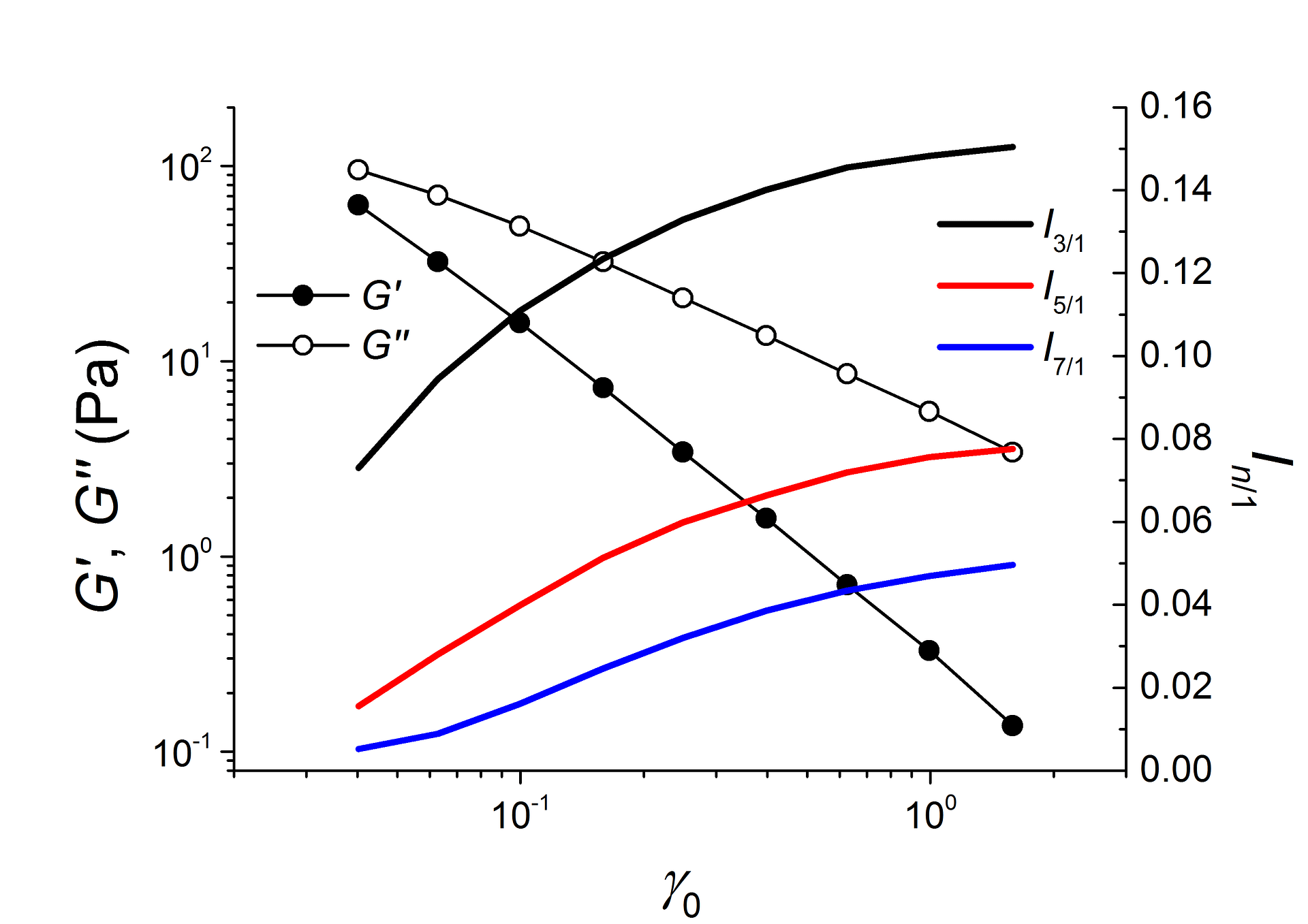
Strain sweep plot of the indicated LAOS parameters
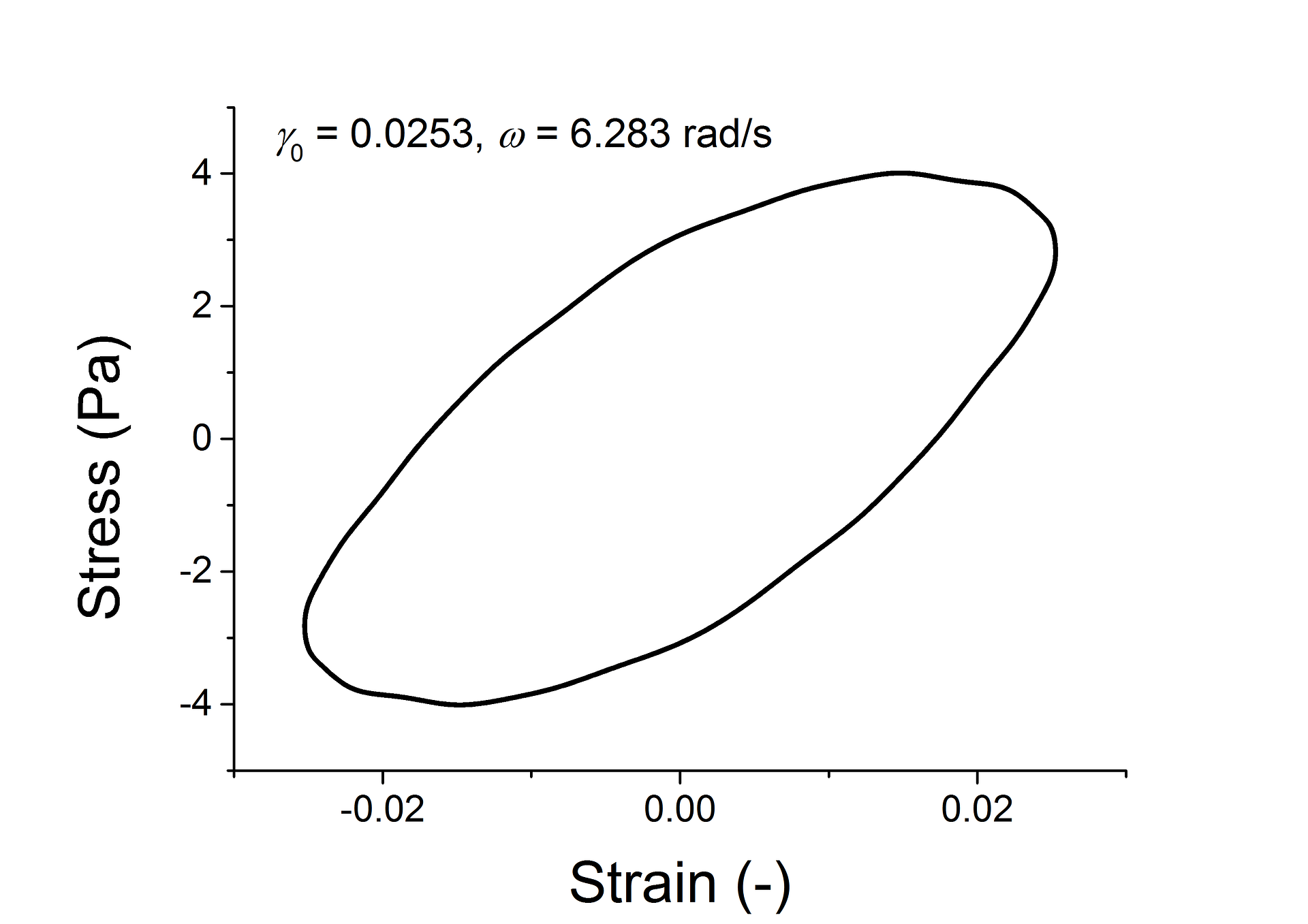
Lissajous curve of the reconstructed data
Please contact me at mswxsun@scut.edu.cn if you encounter any bugs.
References
- K. Hyun, M. Wilhelm, C.O. Klein, K.S. Cho, J.G. Nam, K.H. Ahn, S.J. Lee, R.H. Ewoldt, and G.H. McKinley, "A review of nonlinear oscillatory shear tests: Analysis and application of large amplitude oscillatory shear (LAOS)", Progress in Polymer Science, vol. 36, pp. 1697-1753, 2011. http://dx.doi.org/10.1016/j.progpolymsci.2011.02.002
- W. Sun, Y. Yang, T. Wang, X. Liu, C. Wang, and Z. Tong, "Large amplitude oscillatory shear rheology for nonlinear viscoelasticity in hectorite suspensions containing poly(ethylene glycol)", Polymer, vol. 52, pp. 1402-1409, 2011. http://dx.doi.org/10.1016/j.polymer.2011.01.048